How I Introduce Volumes of Revolution

The two main takeaways from Unit 8 of AP Calculus AB/BC are Accumulation and Volumes of Revolution/Rotation. We finished accumulation a couple of weeks ago and then spent a few days on average value. Last week we began VOLUMES of revolution.

I began by showing them a PowerPoint slideshow of various photos of objects with circular cross-sections and explained that if we put an x-axis through the object and approximated the outline of the object with a function, we could use volumes of revolution to estimate the volume of the object. It is important they realize that this type of volumes is only used to describe 3D objects with a circular cross-section; anything else would be a volume by cross-section (to be learned the next week).

We spend the first day and a half just working the curvy area under the function square root of x from a=0 to b=10. We spend the first day just on various visualizations and manipulatives.

Before we begin volumes, I ask them to recall how we approximated 2D curvy area under a curve. We discuss how we began with Riemann Sums and broke the whole area into smaller rectangular area that we added up to get an estimate. In the end, we added infinite tiny areas to estimate the overall area. The integral is the tool to add infinitely many things. This bolded statement is said again later in the lesson once we are discussing 3D volumes.

I asked them what would happen if we took the curvy area under the square root of x and rotated it around the x-axis - what would that look like? To help them picture this, I have them look in the bins on each group of desks and choose one of these to tape to their pencils.

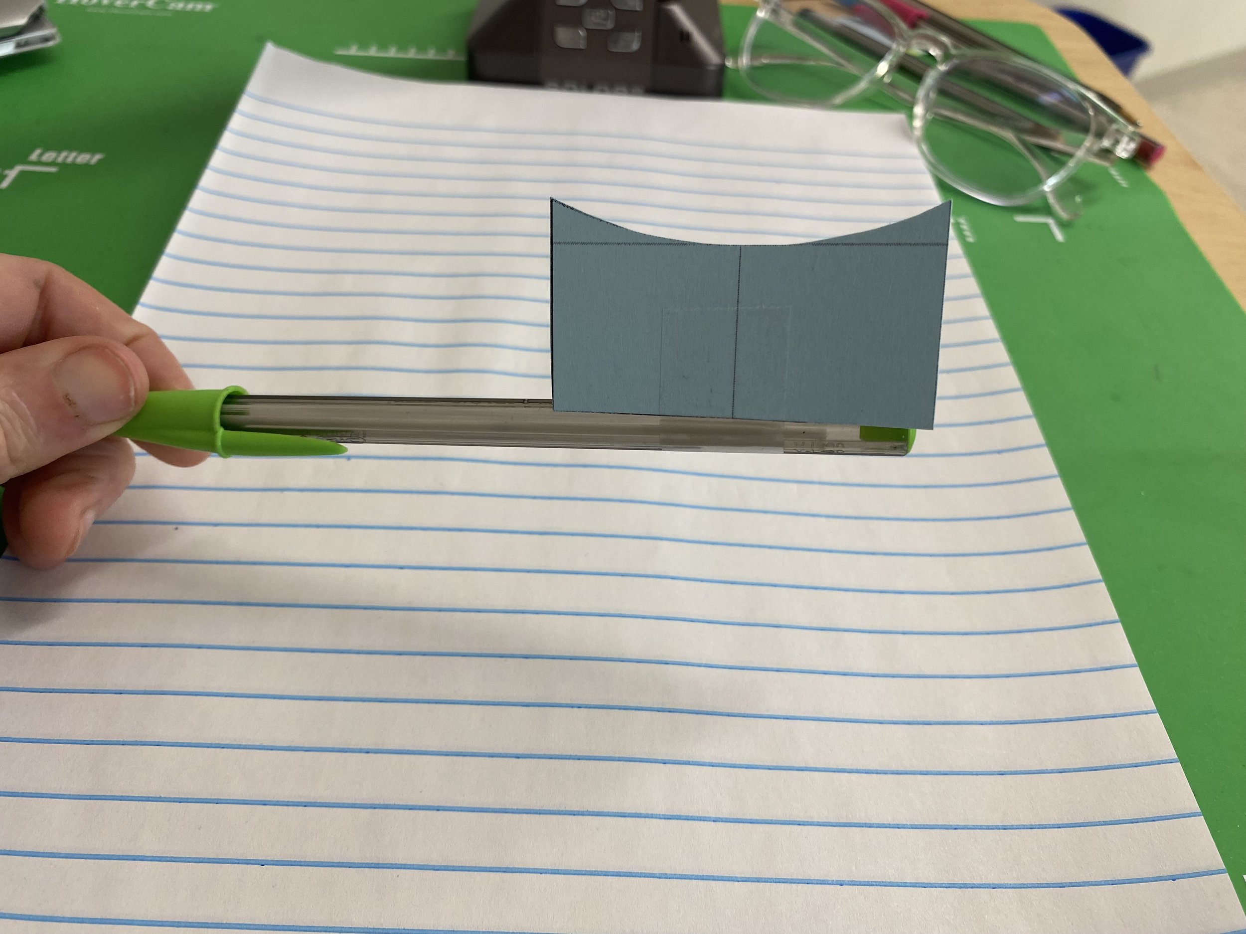
They have 4 different curvy areas to choose from on various colors of cardstock paper. PDF of shapes here.

I tell them to tape their curvy area to their pencil, which is now an x-axis. Then I ask them to spin their curvy area around horizontally to see the 3D volume created. I tell them to spin their pencil as fast as they can until they can REALLY see a 3D volume. We all laugh as we watch each other try to do this; some of them get pretty close to truly seeing a 3D shape. Then I tell them that I can spin my shape faster than any of them can by using my drill - this always gets their attention! I have them get up and gather around the drill to watch it spin the curvy areas and get a great visual of the 3D volume created.

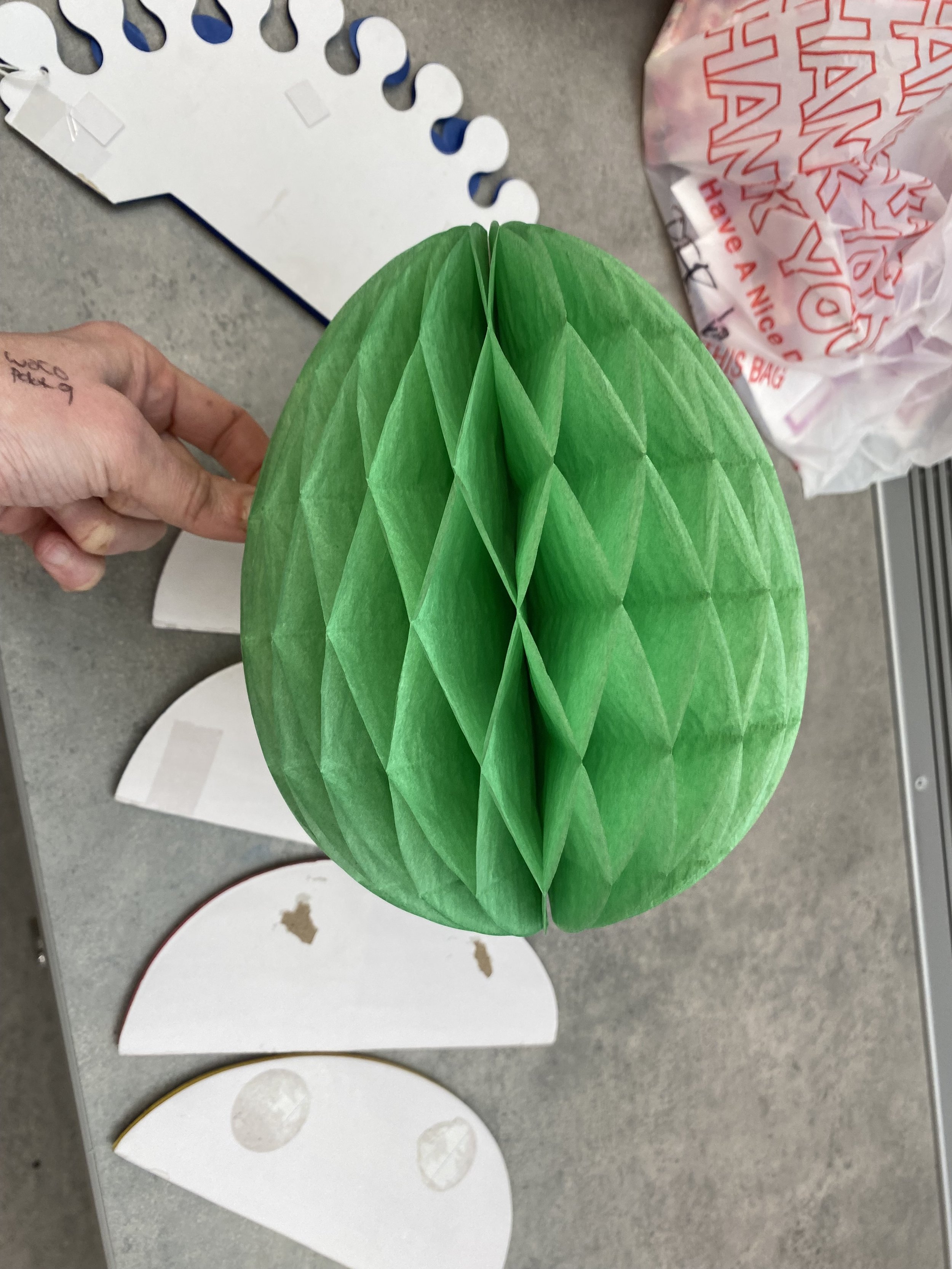
Then I hand out one or two party poppers to each group. We imagine that when folded up, it’s the the curvy area under the square root of x. Then we slowly open up the party popper - essentially revolving the area around the x-axis and watching the volume form.

With the party popper open, I tell them we are going to imagine approximating the volume by chopping it up vertically with a knife. I ask them what shape that would give us and they answer “circles.” I point out that since it will be 3D, they are really cylinders. I ask them to tell me formula for volume of a cylinder - they better remember!

We talk about chopping it up into smaller cylinders, whose volume formula we DO know, and adding up those smaller volumes to get an estimate for the total volume of our 3D shape, which does NOT have an exact volume formula. I ask them how many cylinders we should use to get a REALLY good estimate, and they tell me infinitely many. I repeat the bolded phrase above, but in terms of volume: we will add infinite tiny volumes to estimate the overall volume. The integral is the tool to add infinitely many things.

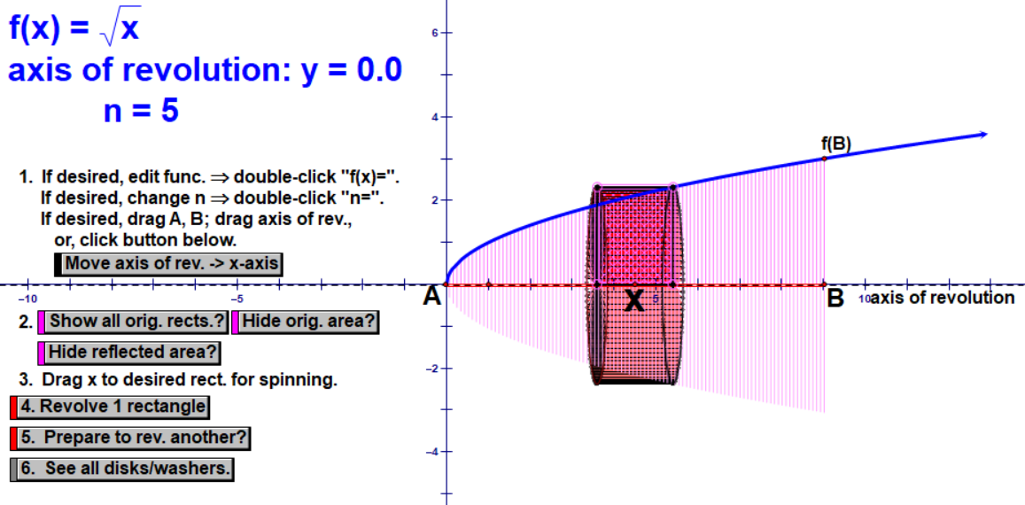
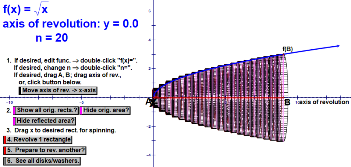
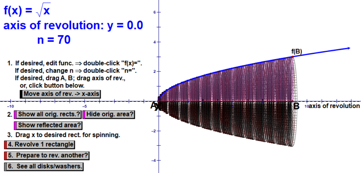
At this point, before getting to the calculus of this, I open up Calculus in Motion, an excellent software tool by Audrey Weeks that uses Geometer’s Sketchpad. I show them the curvy area under square root of x and its reflection under the x-axis. I have them sketch this in their notebooks and do their best to draw a couple cylindrical cross-sections.

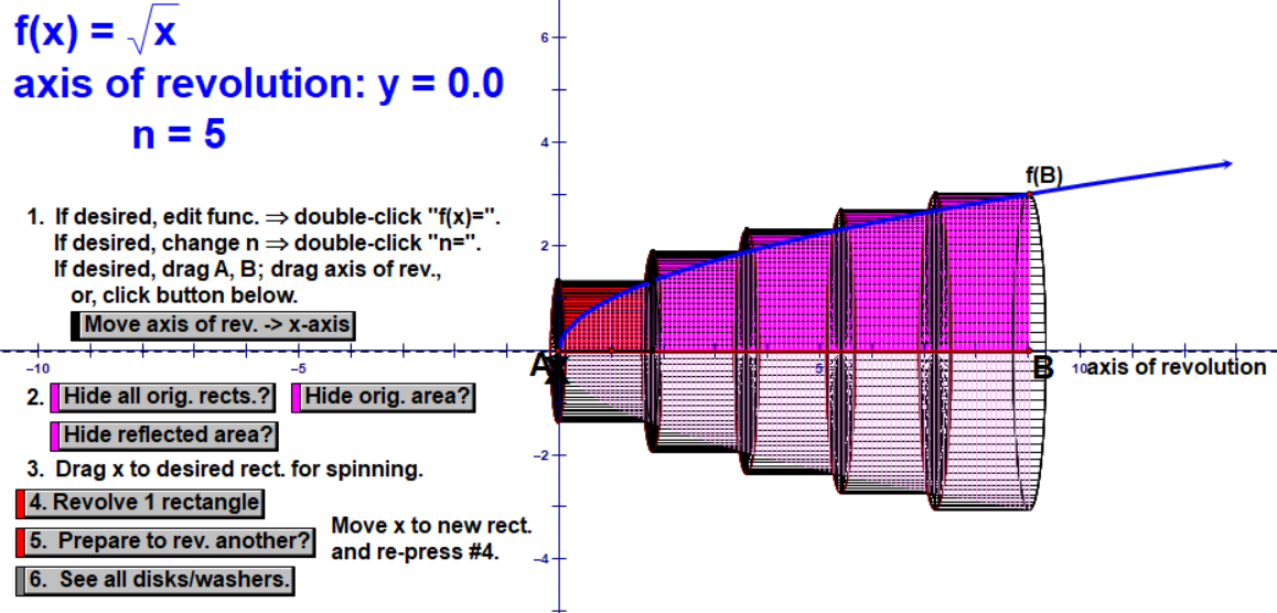
First, we chop it into 5 cylinders. I make a point to emphasize how we are OVER-estimating because our shape is not actually cylindrical, so our cylinders stick out over the top. Then we chop it into 20 and 70 cylinders, noting how the estimate gets closer to the exact volume with less sticking out over the top. We again note that we need infinite cylinders.

I show them the animation of rotating the exact curvy area around the x-axis with no more approximate cylinders. This is what we try to replicate and mark up in our notebooks:

At this point, we are ready to build up the Calculus expression for the exact volume. We begin by writing the volume of a random cylinder using the formula (pi)(r^2)(h). I point out that the height is “sideways,” not up and down, and it is ‘dx’ since it is going to by infinitesimally small. We spend time discussing how we will get an expression for a random radius of any cylinder. This is often the hardest part for them - drawing a random radius and then writing an expression for the length of the radius.

Once we have the expression for a random cylinder, we know that we want to add infinitely many, so just do the integral from a=0 to b=10 of that volume expression! Then they calculate that by hand.

The next day, we change the axis of rotation to be y=-2 so that we have a hollow volume. At this point, I introduce the vocabulary words “disc” and “washer.” We go through how to create a calculus expression for this mew type of volume.

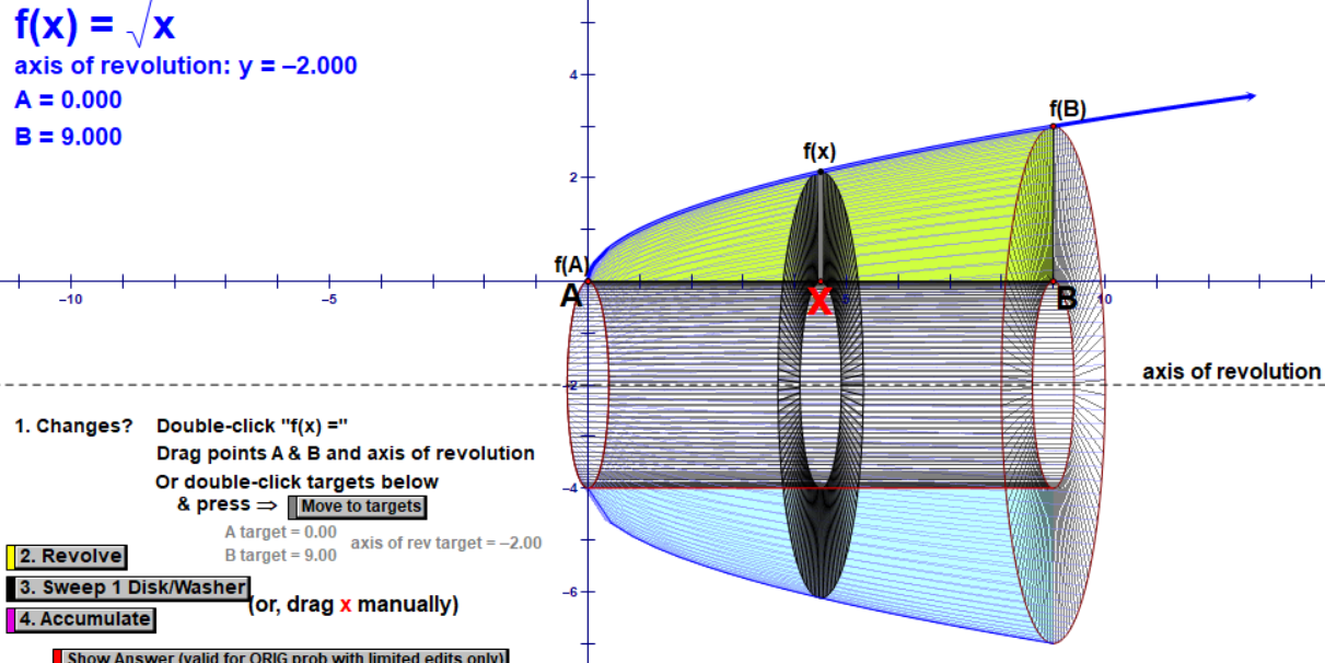
And then they are usually ready to explore fun and different types of volumes, like the one below!